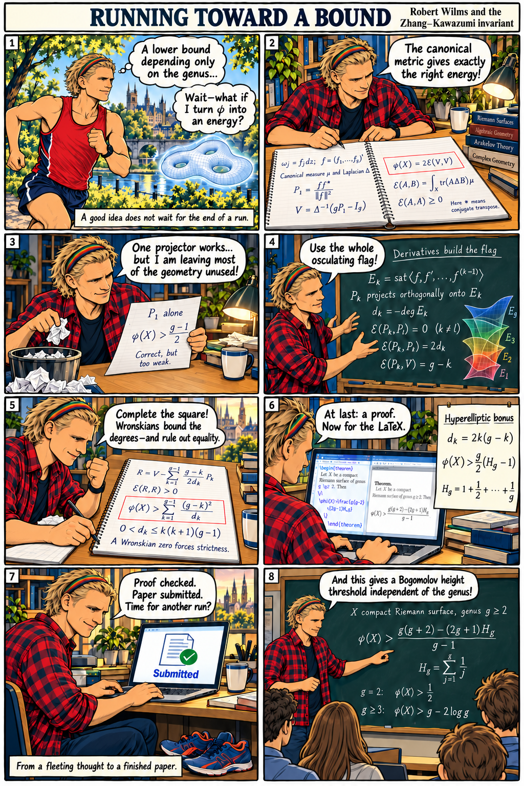
How small can the Zhang–Kawazumi invariant be? An explicit, strict lower bound depending only on the genus, strengthened for hyperelliptic surfaces, gives new lower bounds for canonical arithmetic self-intersections and uniform height thresholds in the Bogomolov conjecture.
For every compact connected Riemann surface X of genus g ≥ 2:
In genus two this gives φ(X) > ½. The argument uses the canonical Arakelov metric and positivity of a bilinear form.
For hyperelliptic X, the stronger bound is φ(X) > (g/2)(Hg−1).
Compare the two bounds
Blue, solid: general. Red, dashed: hyperelliptic. Curves show lower bounds, not values of φ for particular surfaces.
The stable Faltings height of y² = xⁿ − 1, for odd n ≥ 3, is expressed through special values of Euler’s gamma function. Explicit bounds isolate the leading term (n/8) log n and give an upper bound for abelian varieties with the canonical cyclotomic CM-type.
Explore the stable Faltings height of the smooth projective curve Xn: y² = xn − 1, equivalently the height of its Jacobian. The formula applies to odd n ≥ 3, with genus g = (n − 1)/2.
Stable Faltings height · numerical approximationEnable JavaScript to calculate.
Exact value for the chosen n
This finite gamma expression is exact. The decimal and plotted points are numerical evaluations, displayed to eight decimal places. All logarithms are natural.
Formula & normalization
Writing ep = ordp(n), Theorem 1.1 gives
The sum over p runs over prime divisors of n. The exact result above combines the log n term with this prime sum and reduces the rational coefficients.
The normalization is the paper’s: the metric is induced by ⟨η,η′⟩ = (i/2) ∫ η ∧ η̄′. The height is stable, computed after semistable reduction. Γ denotes Euler’s gamma function.
Use integer endpoints 3 ≤ a ≤ b ≤ 10001. Even endpoints are allowed; every odd n in [a,b] is included.
● Prime◆ Prime power (exponent ≥ 2)■ Other composite
Select a point to inspect its exact height above. With the plot focused, use ← and → to move between points; Home and End select the endpoints. The red point is the chosen n.
The bounds and the leading term
−0.975n < hFal(Xn) − (n/8) log n < (9/64)n log log n − 0.263n.
Corollary 1.2 gives these strict bounds. Toggle them to see the lower bound in teal and the upper bound in dashed red. The second vertical-axis option subtracts the leading term to reveal the remaining variation.
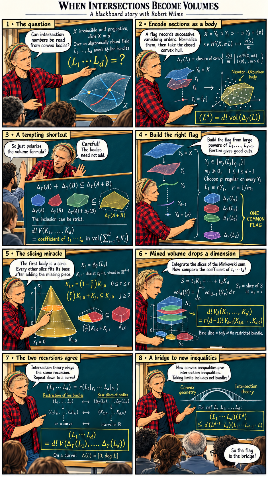
For ample line bundles, a suitable common admissible flag converts their intersection number into the mixed volume of their Newton–Okounkov bodies, with the standard factorial normalization. The flag is built using Bertini’s theorem; slice formulas and convex-geometric calculations drive the proof.
Let L1, …, Ld be ample Q-line bundles on an irreducible projective d-fold over an algebraically closed field. For a suitable admissible flag Y•,
(L1 ··· Ld) = d! V(ΔY•(L1), …, ΔY•(Ld)).
The same flag is used for all bodies. The result does not assert this equality for every flag.
Can Newton–Okounkov bodies turn sums of line bundles into Minkowski sums? An appropriate flag makes this work on two-dimensional subcones of the ample cone; a necessary condition explains the scope of the result, and an application gives an inequality for intersections of nef line bundles.
A non-isotrivial curve of genus g ≥ 2 over a one-dimensional function field, in any characteristic, has at most 16g² + 32g + 124 torsion points in any Abel–Jacobi embedding. More generally, the method bounds the number of points of small Néron–Tate height, using admissible pairings, an arithmetic Hodge index theorem and Green functions on metrized graphs.
Let K = k(B), where k is algebraically closed and B is a smooth projective connected curve. For a smooth projective geometrically connected, non-isotrivial curve X/K of genus g ≥ 2 and any degree-one divisor D,
Differential equations for the Riemann theta function are obtained on Jacobians of Riemann surfaces. The argument develops variants of Fay’s theta identity, guided by corresponding identities in Arakelov theory.
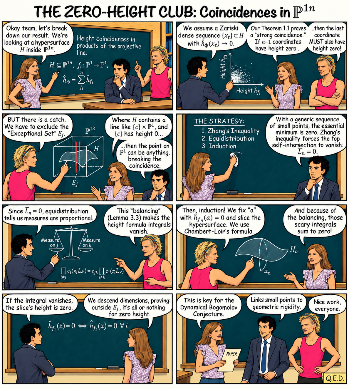
For a hypersurface in a product of projective lines with split dynamics, a generic sequence of small points forces a coincidence: on a suitable dense open subset, the vanishing of n−1 coordinate heights implies the vanishing of all n. The projection and small-point hypotheses are essential; this is a key ingredient in the dynamical Bogomolov conjecture for split maps.
Let K be a number field, or the function field of a smooth projective curve over an algebraically closed field. Let Φ = (f1, …, fn), where each fi : P1K → P1K is a morphism of degree at least 2, and let ĥΦ(x) = ∑ ĥfi(xi). An irreducible hypersurface H ⊂ (P1)n must dominate the product omitting coordinate j and contain a generic sequence whose total canonical height tends to zero.
For x ∈ H(K̄) outside the proper closed locus Ej of complete j-coordinate fibres:
ĥfi(xi) = 0 for every i ≠ j ⇔ ĥΦ(x) = 0.
The comic shows the three-coordinate case. Its “club rules” are exactly the hypotheses above.
How large can the average Arakelov–Green interaction of n points be? An alternative proof of the Faltings–Elkies upper bound gives the order O((log n)/n), with effective constants expressed through bounds in a chosen covering by local coordinates.
A combinatorial calculation of arithmetic intersections on self-products of a curve yields a closed formula for the Néron–Tate heights of tautological cycles in its Jacobian. It also bounds the canonical arithmetic self-intersection in terms of Zhang’s invariant and gives an effective Bogomolov-type result for these cycles.
Let X/K be a smooth projective geometrically connected curve of genus g ≥ 2 with semistable reduction. Fix the canonical degree-one class α = ω/(2g−2), up to torsion. In J = Pic0(X), let
Zm,α = image(Xr → J), (x₁,…,xᵣ) ↦ ∑j=1r mj(xj−α).
Choose nonzero integers mj; negative entries are allowed. The calculator gives exact rational coefficients of the curve’s normalized invariants.
1 ≤ r ≤ g. At r = g, the image is the whole Jacobian and its height is zero.
Exact Néron–Tate height
Enable JavaScript to calculate the exact expression.
Ω = ω̂²/[K:Q], Φ = φ(X)/[K:Q].
Here φ(X) is the global invariant, including the finite-place and complex-embedding contributions. A numerical height also requires Ω and Φ for your curve.
The formula and its normalization
Write S₂ = ∑ mj² and P = ∑j<k mjmk. The choice of α makes hNT(α−ω/(2g−2)) = 0.
h′ℒ(Zm,α) = AΩ + BΦ.
For 2 ≤ r < g:
For r = 1: A = m₁²/[8(g−1)] and B = 0. For r = g: A = B = 0. These separate cases also cover genus two without division by g−2.
ℒ is a symmetric line bundle inducing the canonical principal polarization. The normalization is h′ℒ(Z) = ⟨ℒ̂r+1|Z⟩ / ([K:Q](r+1)⟨ℒr|Z⟩).
High powers of an arithmetically ample hermitian line bundle admit arithmetic divisors whose analytic contribution is arbitrarily small relative to their irreducible classical part. Divisors of small sections also equidistribute towards the curvature measure, giving new results for integer-polynomial zeros and a description of arithmetic intersections through intersections on finite fibres.
For degree n ≥ 1, define the normalized Bombieri height
hB(P) = (1/n) log max0≤k≤n |ak| / √C(n,k).
The paper uses the set
𝒫n,r = {P ∈ Z[X] : deg P = n, hB(P) ≤ r}.
Here r > 0 is a logarithmic bound: the corresponding raw norm radius is enr. Unlike the report’s convention, the leading coefficient must be nonzero.
No sample yet
The sampled polynomial
Choose n and r, then sample a polynomial.
Accumulate up to 100 polynomials under the same n and r. Changing either parameter starts a new collection.
The plot will show numerical approximations to the complex zeros.
Real and imaginary axes use the same scale. Roots are counted with multiplicity; coincident or nearby markers may overlap. The dashed unit circle is a reference.
Numerical zero coordinates
Zero
Real part
Imaginary part
How the sampling works
Put Bk = ⌊enr√C(n,k)⌋. Choose a0, …, an−1 independently and uniformly in −Bk, …, Bk; choose an uniformly from the 2Bn nonzero possibilities. This samples uniformly from the paper’s set. Irreducibility and primitivity are not imposed.
Connection with the distribution theorem
For fixed r > 0, Corollary 1.8 gives convergence on average of the normalized zero measures to the Fubini–Study measure as n grows. More generally, r may vary in a compact subinterval of (0,∞). The theorem concerns increasing degree; one finite sample need not resemble the limit.
Shared experiments retain a repeatable pseudorandom sequence. Accumulation overlays finite numerical zero sets; it does not verify the asymptotic distribution theorem.
This Oberwolfach report describes how zeros of integer polynomials distribute when coefficients satisfy weighted bounds. The limiting measure is the Fubini–Study measure on the projective line; the experiment below displays finite samples with the report’s precise coefficient convention.
This set includes the zero polynomial, constants and polynomials of degree below n. Here C(n,k) = n!/[k!(n−k)!].
No sample yet
The sampled polynomial
Choose n and r, then sample a polynomial.
Accumulate up to 100 polynomials under the same n and r. Changing either parameter starts a new collection.
The plot will show numerical approximations to the complex zeros.
Real and imaginary axes use the same scale. Roots are counted with multiplicity; coincident or nearby markers may overlap. The dashed unit circle is a reference.
Numerical zero coordinates
Zero
Real part
Imaginary part
How the sampling works
Each coefficient ak is chosen independently and uniformly from the integers −Bk, …, Bk, where Bk = ⌊r√C(n,k)⌋. Thus every member of 𝒫n,r has the same sampling probability. We keep zero and degree drops instead of drawing again.
Connection with the distribution theorem
The report proves convergence on average of normalized zero measures to the Fubini–Study measure when 1 < lim inf rn1/n ≤ lim sup rn1/n < ∞. A fixed raw radius does not satisfy this hypothesis. The related paper’s sampler uses a logarithmic parameter instead.
Shared experiments retain a repeatable pseudorandom sequence. Accumulation overlays finite numerical zero sets; it does not verify the asymptotic distribution theorem.
The degeneration of the norm of the theta function is described using the polarized real torus attached to a degenerating family of abelian varieties. For curves this yields the asymptotics of the Zhang–Kawazumi invariant in terms of a metrized reduction graph, leading to uniform lower bounds for heights on tautological cycles.
Theta-function integrals give explicit formulas for Faltings’ delta invariant, a lower bound depending only on the genus, and an upper bound for the Arakelov–Green function. The delta and Zhang–Kawazumi invariants also acquire canonical extensions to indecomposable principally polarized complex abelian varieties.
This Oberwolfach report presents explicit formulas for Faltings’ delta invariant and their role in Arakelov geometry. It offers a short entry point to the theta-function formulas and bounds developed in the related research paper.
The doctoral thesis develops explicit formulas for the delta invariant in Arakelov geometry, connecting analytic invariants of Riemann surfaces with theta functions and arithmetic geometry. Completed at the University of Bonn in 2016 under the supervision of Gerd Faltings.
2011 · PublishedNumber theory
The family of ternary cyclotomic polynomials with one free prime
How do the coefficients of Φₚᵩᵣ change when two odd primes p < q are fixed and the third prime r varies? This paper establishes results and formulates conjectures for this family of ternary cyclotomic polynomials, among the simplest cyclotomic families whose coefficient behaviour is not fully understood.
Lines indicate mathematical connections, rather than a chronology or a claim that one theorem implies another.
01 / Diophantine geometry
How small can a height be?
ĥf(f(x)) = deg(f) ĥf(x)
Canonical heights make arithmetic complexity compatible with dynamics. With Mavraki and Schmidt, I study when zero heights in different coordinates must coincide.
With Looper and Silverman, I give a uniform quantitative Manin–Mumford bound for non-isotrivial curves over function fields.
Canonical metrics, Green functions and theta functions bring the complex fibres into arithmetic intersection theory.
My work on Faltings’ delta-invariant and the Zhang–Kawazumi invariant turns these analytic quantities into explicit formulas and uniform arithmetic bounds.
Valuations send sections to lattice points. Newton–Okounkov bodies record their asymptotic growth.
For ample Q-line bundles, a suitable common flag makes mixed volumes recover intersection numbers. ECO functions extend the viewpoint of bounded algebraic complexity.
 Read the comic ↗